Manifold Learning Techniques#

Creator : Mahdieh Alizadeh
Email address: Mahdieh20201@gmail.com
Machine Learning 1403-fall
In manifold learning, we aim to uncover the low-dimensional structure embedded in high-dimensional data. Here, we discuss two popular methods: Multidimensional Scaling (MDS) and Isomap.
1. Multidimensional Scaling (MDS)#
Short Description: MDS aims to preserve pairwise distances between data points by embedding them in a lower-dimensional space. This approach uses the concept of stress minimization to maintain distance relationships.
Mathematical Formulation#
The objective function for classical MDS is given by:
\( \text{minimize}_{\{y_i\}_{i=1}^n} c_1 = \sum_{i=1}^n \sum_{j=1}^n (x_i^T x_j - y_i^T y_j)^2, \)
whose matrix form is:
\( \text{minimize}_Y \, c_1 = \| X^T X - Y^T Y \|_F^2, \)
where \( (|\cdot\|_F)\) denotes the Frobenius norm.
The eigenvalue decomposition of the Gram matrix \(( X^T X )\) is:
\( X^T X = V \Delta V^T, \quad Y^T Y = Q \Psi Q^T \)
The objective function can be simplified as:
\( \| X^T X - Y^T Y \|_F^2 = \text{tr}[(X^T X - Y^T Y)^T (X^T X - Y^T Y)] = \text{tr}[(X^T X - Y^T Y)(X^T X - Y^T Y)] = \text{tr}[(X^T X - Y^T Y)^2], \)
where \(\text{tr}(\cdot)\) denotes the trace of the matrix. If \(X^T X\) and \(Y^T Y\) are decomposed using eigenvalue decomposition, the result is:
\( X^T X = V \Lambda V^T, \)
\( Y^T Y = Q \Psi Q^T, \)
where the eigenvectors are sorted from leading (largest eigenvalue) to trailing (smallest eigenvalue). Note that, rather than eigenvalue decomposition of \(X^T X\) and \(Y^T Y\), it is possible to decompose \(X\) and \(Y\) using a Singular Value Decomposition (SVD) and by taking the right singular vectors of \(X\) and \(Y\) as \(V\) and \(Q\), respectively.
the matrices \(\Delta\) and \(\Psi\) are obtained by squaring the singular values (to power 2).
The objective function can be further simplified as:
\( \| X^T X - Y^T Y \|_F^2 = \text{tr}[(X^T X - Y^T Y)^2] = \text{tr}[(V \Delta V^T - Q \Psi Q^T)^2] = \text{tr}[(V \Delta V^T - V V^T Q \Psi Q^T V V^T)^2] = \text{tr}[(\Delta - V^T Q \Psi Q^T V)^2] \)
where these are for \(V^T V = VV^T = I\) because \(V\) is a nontruncated (square) orthogonal matrix (where \(I\) denotes the identity matrix). The reason is the cyclic property of the trace operator.
If \(\mathbb{R}^{n \times n} \ni M := V^T Q\), then:
\( \| X^T X - Y^T Y \|_F^2 = \text{tr}[(\Delta - M \Psi M^T)^2]. \)
Therefore:
\( \text{minimize}_Y \| X^T X - Y^T Y \|_F^2 = \text{minimize}_{M, Y} \text{tr}[(\Delta - M \Psi M^T)^2]. \)
This means that the objective function is:
\( c_1 = \text{tr}[(\Delta - M \Psi M^T)^2] = \text{tr}(\Delta^2 + (M \Psi M^T)^2 - 2 \Delta M \Psi M^T) = \text{tr}(\Delta^2) + \text{tr}((M \Psi M^T)^2) - 2 \text{tr}(\Delta M \Psi M^T). \) As the optimization problem is unconstrained and the objective function is the trace of a quadratic function, the minimum is nonnegative.
If the derivative with respect to the first objective variable, i.e., \(M\), is taken, then the result is:
\( \mathbb{R}^{n \times n} \ni \frac{\partial c_1}{\partial M} = 2(M \Psi M^T) M - 2 \Delta M \Psi = 0 \Rightarrow (M \Psi M^T) (M) = (\Delta) (M \Psi M^T) \)
(a)
\( M \Psi M^T = \Delta, \)
where (a) is because \(M \neq 0\). Both Eqs are:
\( M \Psi M^T = \Delta, \)
whose one possible solution is:
\( M = I, \)
\( \Psi = \Delta. \)
which means that the minimum value of the nonnegative objective function \(\text{tr}((\Delta - M \Psi M^T)^2)\) is zero.
If there is \(M = V^T Q\), there is:
\( \therefore V^T Q = I \Rightarrow Q = V. \)
there is:
\( Y^T Y = Q \Psi Q^T = Q \Psi^{\frac{1}{2}} Q^T Q \Psi^{\frac{1}{2}} Q^T \Rightarrow Y = \Psi^{\frac{1}{2}} Q^T. \)
from sklearn.datasets import make_s_curve
from scipy.spatial.distance import pdist, squareform
from sklearn.datasets import load_digits
import matplotlib.pyplot as plt
import numpy as np


# Parameters
n_samples = 300
random_state = 0
embedding_dim = 2  # Target dimensionality for MDS

# Generate the S-curve dataset
S_points, _ = make_s_curve(n_samples, random_state=random_state)

# Compute the Euclidean distance matrix
D = squareform(pdist(S_points, metric='euclidean'))

# Centering matrix
n = D.shape[0]
H = np.eye(n) - np.ones((n, n)) / n

# Double centering the squared distance matrix
D_squared = D ** 2
B = -0.5 * H @ D_squared @ H

# Eigen decomposition of the centered matrix
eigenvalues, eigenvectors = np.linalg.eigh(B)

# Sort eigenvalues and corresponding eigenvectors in descending order
sorted_indices = np.argsort(eigenvalues)[::-1]
eigenvalues = eigenvalues[sorted_indices]
eigenvectors = eigenvectors[:, sorted_indices]

# Select the top `embedding_dim` eigenvalues and eigenvectors
Lambda_m = np.diag(np.sqrt(eigenvalues[:embedding_dim]))
Q_m = eigenvectors[:, :embedding_dim]

# Compute the low-dimensional embedding
X_transformed = Q_m @ Lambda_m

# Plotting the result
plt.figure(figsize=(8, 6))
plt.scatter(X_transformed[:, 0], X_transformed[:, 1], c=S_points[:, 1], cmap='viridis', s=15, alpha=0.7)
plt.colorbar(label="Original Y-axis position (as color gradient)")
plt.xlabel("MDS Component 1")
plt.ylabel("MDS Component 2")
plt.title("Classical MDS Projection of S-curve Dataset")
plt.show()

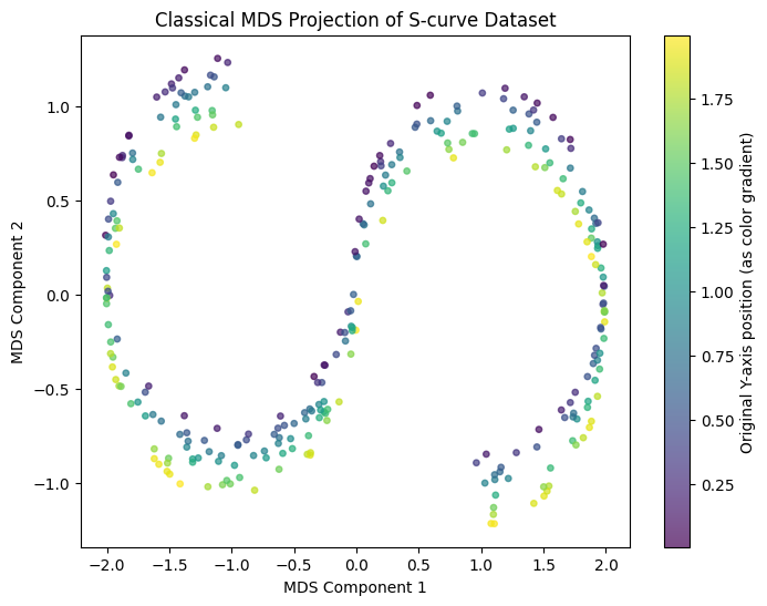
Classical MDS Implementation on S-curve Dataset#
This code applies Classical Multidimensional Scaling (MDS) to reduce a 3D S-curve dataset to 2D while preserving pairwise distances. It calculates the Euclidean distance matrix, centers the squared distances, and performs eigendecomposition to extract the top two eigenvalues and eigenvectors, forming a 2D embedding. The result is visualized with colors representing the original Y-axis values, capturing the S-curve structure in 2D.
# Load digits dataset and select a subset of samples
x, y = load_digits(return_X_y=True)
samples = 300  # Number of samples to use
x_subset = x[:samples]
y_subset = y[:samples]

# Compute the Euclidean distance matrix for the subset
D = squareform(pdist(x_subset, metric='euclidean'))

# Centering matrix
n = D.shape[0]
H = np.eye(n) - np.ones((n, n)) / n

# Double-center the squared distance matrix
D_squared = D ** 2
B = -0.5 * H @ D_squared @ H

# Eigen decomposition of the centered matrix
eigenvalues, eigenvectors = np.linalg.eigh(B)

# Sort eigenvalues and corresponding eigenvectors in descending order
sorted_indices = np.argsort(eigenvalues)[::-1]
eigenvalues = eigenvalues[sorted_indices]
eigenvectors = eigenvectors[:, sorted_indices]

# Select the top `m` eigenvalues and eigenvectors
m = 2  # Target dimensionality for MDS
Lambda_m = np.diag(np.sqrt(eigenvalues[:m]))
Q_m = eigenvectors[:, :m]

# Compute the low-dimensional embedding
X_transformed = Q_m @ Lambda_m

# Plotting the result
plt.figure(figsize=(8, 6))
scatter = plt.scatter(X_transformed[:, 0], X_transformed[:, 1], c=y_subset, cmap='tab10', alpha=0.7)
plt.colorbar(scatter, label="Digit Label")
plt.xlabel("MDS Component 1")
plt.ylabel("MDS Component 2")
plt.title("Classical MDS Projection of Digits Dataset (300 samples)")
plt.show()

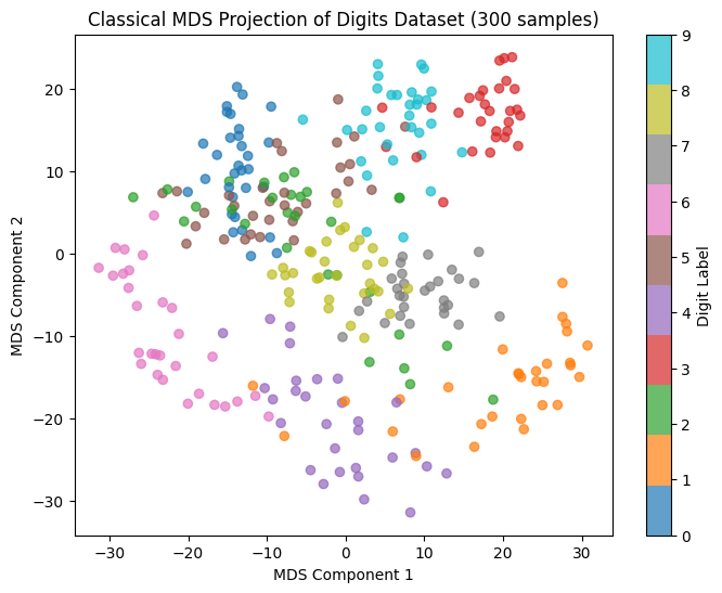
Classical MDS Implementation on digits Dataset#
This code performs Classical Multidimensional Scaling (MDS) on a subset of the digits dataset, projecting high-dimensional data into 2D to maintain relative distances between samples. It first calculates pairwise Euclidean distances and uses a centering matrix to create a Gram matrix suitable for dimensionality reduction. After eigendecomposition, the top two components are selected to construct a 2D representation. The final visualization shows each digit as a color-coded point, highlighting patterns and clusters in the reduced space, which aids in understanding the dataset’s structure and relationships among digit samples.
2. Isometric Mapping (Isomap)#
Isomap is a special case of the generalized classical MDS, where instead of using Euclidean distances, the geodesic distance is used:
\( D_{ij}^{(g)} = \min \sum_{i=2}^{l} \| r_i - r_{i-1} \|_2, \)
where \(( l \geq 2 )\) is the length of the sequence of points \( ( r_i \in \{x_i\}_{i=1}^l )\), and \(( D_{ij}^{(g)} )\) denotes the geodesic distance matrix.
Isomap’s formulation involves a kernel matrix based on the geodesic distance:
\( K = -\frac{1}{2} H D^{(g)} H \)
where \(( D^{(g)} )\) is the geodesic distance matrix, and \(( H )\) is the centering matrix.
ISOMAP on S-curve dataset#
This code applies the Isomap algorithm to reduce a 3D S-curve dataset to 2D while preserving its shape.
Calculate Distances between all data points.
Build Graph by connecting each point to its closest
n_neighbors.Compute Geodesic Distances along the graph to approximate the manifold structure.
Eigenvalue Decomposition extracts the top features, yielding the final 2D embedding.
The result is a 2D plot showing the S-curve’s shape and continuity in reduced dimensions.
import numpy as np
from scipy.spatial import distance_matrix
from scipy.sparse.csgraph import shortest_path
from scipy.linalg import eigh
from sklearn.datasets import make_s_curve
import matplotlib.pyplot as plt

def isomap(data, n_neighbors=5, n_components=2):
    # Step 1: Compute the pairwise Euclidean distance matrix
    distances = distance_matrix(data, data)

    # Step 2: Build the neighborhood graph
    n_samples = data.shape[0]
    neighborhood_graph = np.full((n_samples, n_samples), np.inf)

    # Connect each point to its k nearest neighbors
    for i in range(n_samples):
        nearest_neighbors = np.argsort(distances[i])[:n_neighbors + 1]  # +1 includes the point itself
        neighborhood_graph[i, nearest_neighbors] = distances[i, nearest_neighbors]

    # Step 3: Compute shortest paths (geodesic distances)
    geodesic_distances = shortest_path(neighborhood_graph, method='D', directed=False)

    # Step 4: Double-center the geodesic distance matrix
    n = geodesic_distances.shape[0]
    h = np.eye(n) - np.ones((n, n)) / n
    b = -0.5 * h @ (geodesic_distances ** 2) @ h

    # Step 5: Compute the top eigenvalues and eigenvectors
    eigvals, eigvecs = eigh(b, eigvals=(n - n_components, n - 1))  # Get largest n_components eigenvalues
    indices = np.argsort(eigvals)[::-1]  # Sort in descending order
    eigvals, eigvecs = eigvals[indices], eigvecs[:, indices]

    # Step 6: Compute the coordinates in the reduced space
    embedding = eigvecs * np.sqrt(eigvals)

    return embedding[:, :n_components]

# Generate the S-curve dataset
data, color = make_s_curve(n_samples=1000, noise=0.05)

# Apply ISOMAP
reduced_data = isomap(data, n_neighbors=10, n_components=2)

# Plot the result
plt.scatter(reduced_data[:, 0], reduced_data[:, 1], c=color, cmap='viridis')
plt.colorbar()
plt.xlabel('Component 1')
plt.ylabel('Component 2')
plt.title('ISOMAP Projection of the S-Curve')
plt.show()
---------------------------------------------------------------------------
TypeError                                 Traceback (most recent call last)
Cell In[3], line 43
     40 data, color = make_s_curve(n_samples=1000, noise=0.05)
     42 # Apply ISOMAP
---> 43 reduced_data = isomap(data, n_neighbors=10, n_components=2)
     45 # Plot the result
     46 plt.scatter(reduced_data[:, 0], reduced_data[:, 1], c=color, cmap='viridis')

Cell In[3], line 30, in isomap(data, n_neighbors, n_components)
     27 b = -0.5 * h @ (geodesic_distances ** 2) @ h
     29 # Step 5: Compute the top eigenvalues and eigenvectors
---> 30 eigvals, eigvecs = eigh(b, eigvals=(n - n_components, n - 1))  # Get largest n_components eigenvalues
     31 indices = np.argsort(eigvals)[::-1]  # Sort in descending order
     32 eigvals, eigvecs = eigvals[indices], eigvecs[:, indices]

TypeError: eigh() got an unexpected keyword argument 'eigvals'
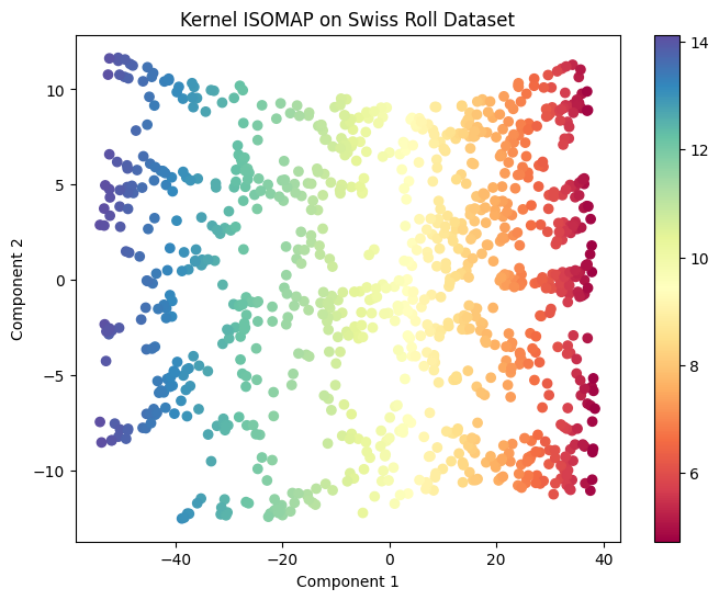
Kernel ISOMAP#
Kernel Isomap extends the original by using kernel methods on the geodesic distance matrix:
\( K(D^2) = -\frac{1}{2} H D^2 H \)
And a modified kernel \(( K' ) \) is defined as:
\( K' = K(D^2) + 2cK(D) + \frac{1}{c} H, \)
where \(( c \geq c^* )\), and \(( c^* )\) is the largest eigenvalue of the matrix:
\( \begin{bmatrix} 0 & 2K(D^2) \\ -4K(D^2) & 0 \end{bmatrix}. \)
For out-of-sample embedding, Isomap uses kernel mapping. Consider a mapping of any data point:
\( y(x) = \sum_{j=1}^{n} \alpha_j k(x, x_j), \) where \(( k(x, x_j) ) \) is a Gaussian kernel:
\( k(x, x_j) = \exp\left( -\frac{\| x - x_j \|^2}{2 \sigma_j^2} \right), \)
and \( ( \sigma_j )\) is defined as:
\( \sigma_j := \gamma \times \min_i \| x_j - x_i \|_2, \)
where \(( \gamma )\) is a small positive number. The objective is to minimize the following cost function to obtain the out-of-sample points:
\( \text{minimize} \sum_{i=1}^{n} \| y_i - y(x_i) \|_2^2. \)
The corresponding kernel matrix is defined as:
\( K'(i,j) = \frac{k(x_i^{(t)}, x_j)}{\sum_{l=1}^{n} k(x_l^{(t)}, x_j)}, \)
where \(( x_i^{(t)} )\) is the \(( i )th \) out-of-sample data point.
import numpy as np
from scipy.spatial import distance_matrix
from scipy.linalg import eigh
from sklearn.neighbors import NearestNeighbors
from scipy.sparse.csgraph import shortest_path
import matplotlib.pyplot as plt
from sklearn.datasets import make_swiss_roll

def nearest_neighbor_graph(X, n_neighbors):
    nbrs = NearestNeighbors(n_neighbors=n_neighbors).fit(X)
    distances, indices = nbrs.kneighbors(X)

    # Create the graph
    n_samples = X.shape[0]
    graph = np.full((n_samples, n_samples), np.inf)

    for i in range(n_samples):
        for j in range(n_neighbors):
            graph[i, indices[i, j]] = distances[i, j]
            graph[indices[i, j], i] = distances[i, j]

    return graph

def compute_geodesic_distances(graph):
    return shortest_path(graph, method='auto', directed=False)

def center_distance_matrix(D):
    n = D.shape[0]
    H = np.eye(n) - (1/n) * np.ones((n, n))
    K = -0.5 * H @ (D ** 2) @ H
    return K

def compute_eigen(K, p):
    eigvals, eigvecs = eigh(K)
    sorted_indices = np.argsort(eigvals)[::-1]
    eigvals = eigvals[sorted_indices]
    eigvecs = eigvecs[:, sorted_indices]
    eigvals = eigvals[:p]
    eigvecs = eigvecs[:, :p]
    return eigvals, eigvecs

def compute_embedding(eigvals, eigvecs):
    Y = eigvecs @ np.diag(np.sqrt(eigvals))
    return Y

def kernel_isomap(X, n_neighbors, p):
    # Step 1: Construct the kNN graph
    graph = nearest_neighbor_graph(X, n_neighbors)
    # Step 2: Compute the geodesic distances
    D_geodesic = compute_geodesic_distances(graph)
    # Step 3: Center the geodesic distance matrix
    K = center_distance_matrix(D_geodesic)
    # Step 4: Compute the top p eigenvalues and eigenvectors
    eigvals, eigvecs = compute_eigen(K, p)
    # Step 5: Compute the embedding
    Y = compute_embedding(eigvals, eigvecs)
    return Y

# Generate the Swiss roll dataset
n_samples = 1000
X, color = make_swiss_roll(n_samples=n_samples, noise=0.05,random_state=48)
# Apply Kernel ISOMAP
n_neighbors = 10
p = 10
Y = kernel_isomap(X, n_neighbors, p)
# Plot the results
plt.figure(figsize=(8, 6))
plt.scatter(Y[:, 0], Y[:, 1], c=color, cmap=plt.cm.Spectral)
plt.title("Kernel ISOMAP on Swiss Roll Dataset")
plt.xlabel("Component 1")
plt.ylabel("Component 2")
plt.colorbar()
plt.show()

References#
Ghojogh, B., Crowley, M., Karray, F., & Ghodsi, A. (2023). Elements of Dimensionality Reduction and Manifold Learning. Springer
