What is Projection?

What is Projection?#

Author : Mustafa Sadeghi
Contact : mustafasadeghi@mail.um.ac.ir

Definition of Projection in $R^{2}$ #

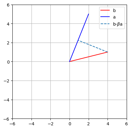
The projection of a vector $\vec{b}$ onto another vector $\vec{a}$ is the component of $\vec{b}$ that lies along the direction of $\vec{a}$ . This projection represents the closest vector along the line defined by $\vec{a}$ to the vector $\vec{b}$ . The projection minimizes the difference between $\vec{b}$ and its projection, making the residual orthogonal to $\vec{a}$ . The formula for the projection of $\vec{b}$ onto $\vec{a}$ is:

{Proj}_{\vec{a}} (\vec{b}) = \frac{{\vec{a}}^{T} \vec{b}}{{\vec{a}}^{T} \vec{a}} \vec{a}

Geometric Implementation

In this formula:

${\vec{a}}^{T} \vec{b}$ represents the dot product of $\vec{b}$ and $\vec{a}$ , which measures how much $\vec{b}$ aligns with $\vec{a}$ .
${\vec{a}}^{T} \vec{a}$ represents the magnitude (length) of vector $\vec{a}$ , ensuring that the projection accounts for the size of $\vec{a}$ .
The result is a scaled version of $\vec{a}$ that points in the same direction as $\vec{a}$ , but has a magnitude such that the difference between $\vec{b}$ and its projection is minimized.

In summary, projection is the transformation that gives the closest vector along the direction of $\vec{a}$ to $\vec{b}$ , ensuring orthogonality between the residual and $\vec{a}$ .

import numpy as np
import matplotlib.pyplot as plt
import math

# line b
b = np.array([ 4,1 ])

# line a
a = np.array([ 2, 5 ])

# beta
beta = (a.T@b) / (a.T@a)

# draw!
plt.plot([0, b[0]],[0, b[1]],'r',label='b')
plt.plot([0, a[0]],[0, a[1]],'b',label='a')

# now plot projection line
plt.plot([b[0], beta*a[0]],[b[1], beta*a[1]],'--',label=r'b-$\beta$a')
plt.axis('square')
plt.grid()
plt.legend()
plt.axis((-6, 6, -6, 6))

plt.show()

../_images/361ae4352228b938d5630f2fcdf2b01bf0c0a72b52935b862160a13c947ba821.png

Projection Derivation#

Start with the condition for projection:

{\vec{a}}^{T} (\vec{b} - \vec{a} β) = 0

This states that the vector $\vec{b} - \vec{a} β$ , which represents the error between $\vec{b}$ and its projection onto $\vec{a}$ , must be orthogonal to $\vec{a}$ .

Expand and rearrange:

{\vec{a}}^{T} \vec{b} - {\vec{a}}^{T} \vec{a} β = 0

Solve for $β$ :

{\vec{a}}^{T} \vec{a} β = {\vec{a}}^{T} \vec{b}

β = \frac{{\vec{a}}^{T} \vec{b}}{{\vec{a}}^{T} \vec{a}}

Thus, the scalar $β$ is the factor by which $\vec{a}$ is scaled to give the projection of $\vec{b}$ onto $\vec{a}$ .

Finally, the projection of $\vec{b}$ onto $\vec{a}$ is given by:

{Proj}_{\vec{a}} (\vec{b}) = β \vec{a} = \frac{{\vec{a}}^{T} \vec{b}}{{\vec{a}}^{T} \vec{a}} \vec{a}

notice : $β \vec{a}$ is as close as possible to point b withuot living the line a.

Projection methods in $R^{2}$ (vector to vector)#

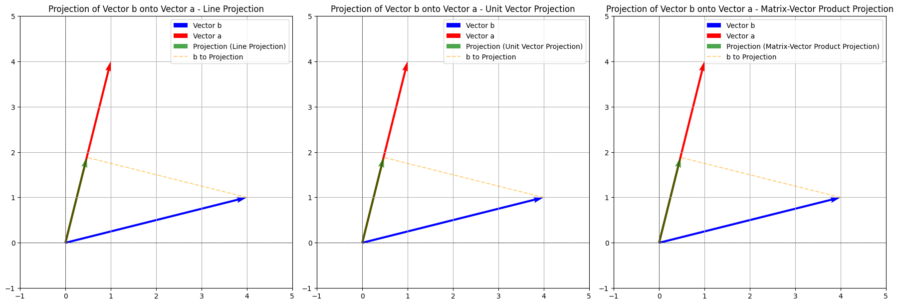
Projection of Vector $\vec{b} = [4, 1]$ onto $\vec{a} = [1, 4]$ #

Method 1: Projection onto a Line#

The projection of $\vec{b}$ onto a line defined by $\vec{a}$ is calculated as:

{Proj}_{a} (\vec{b}) = (\frac{\vec{b} \cdot \vec{a}}{\vec{a} \cdot \vec{a}}) \vec{a}

Steps:

Dot product of $\vec{b} \cdot \vec{a}$ :

$\vec{b} \cdot \vec{a} = (4) (1) + (1) (4) = 4 + 4 = 8$

This step finds the magnitude of the projection of $\vec{b}$ in the direction of $\vec{a}$ .
Dot product of $\vec{a} \cdot \vec{a}$ :

$\vec{a} \cdot \vec{a} = (1) (1) + (4) (4) = 1 + 16 = 17$

This calculates the magnitude of vector $\vec{a}$ , which helps in scaling the projection correctly.
Scalar $β$ :

$β = \frac{8}{17}$

The ratio of the dot products gives the scalar that determines how much of $\vec{a}$ is in the direction of $\vec{b}$ .
Final projection:

${Proj}_{a} (\vec{b}) = \frac{8}{17} \times [1, 4] = [\frac{8}{17}, \frac{32}{17}] \approx [0.47, 1.88]$

The vector $\vec{a}$ is scaled by $β$ to get the projection.

Method 2: Projection Using a Unit Vector#

In this method, we first normalize $\vec{a}$ to create a unit vector, then calculate the projection.

Steps:

Normalize $\vec{a}$ :

$‖ \vec{a} ‖ = \sqrt{(1)^{2} + (4)^{2}} = \sqrt{17}, \hat{u} = \frac{1}{\sqrt{17}} [1, 4]$

This step ensures that the projection is independent of the magnitude of $\vec{a}$ , focusing only on the direction.
Dot product of $\vec{b} \cdot \hat{u}$ :

$\vec{b} \cdot \hat{u} = 4 \times \frac{1}{\sqrt{17}} + 1 \times \frac{4}{\sqrt{17}} = \frac{8}{\sqrt{17}}$

This calculates the component of $\vec{b}$ in the direction of the unit vector $\hat{u}$ .
Final projection:

${Proj}_{a} (\vec{b}) = \frac{8}{\sqrt{17}} \times [\frac{1}{\sqrt{17}}, \frac{4}{\sqrt{17}}] = [\frac{8}{17}, \frac{32}{17}] \approx [0.47, 1.88]$

The projection is obtained by scaling the unit vector $\hat{u}$ .

Method 3: Projection as a Linear Transformation#

Since projections are linear transformations, they can also be expressed as a matrix-vector multiplication.

Steps:

Unit vector $\hat{u}$ : From Method 2, the unit vector is:

$\hat{u} = [\frac{1}{\sqrt{17}}, \frac{4}{\sqrt{17}}]$
Construct the projection matrix $A$ :

$\begin{array}{r} A = [\begin{array}{c} u_{1}^{2} & u_{1} u_{2} \\ u_{1} u_{2} & u_{2}^{2} \end{array}] = [\begin{array}{c} \frac{1}{17} & \frac{4}{17} \\ \frac{4}{17} & \frac{16}{17} \end{array}] \end{array}$

This matrix represents the transformation that projects any vector onto the line defined by $\hat{u}$ .
Matrix multiplication:

$\begin{array}{r} A \vec{b} = [\begin{array}{c} \frac{1}{17} & \frac{4}{17} \\ \frac{4}{17} & \frac{16}{17} \end{array}] [\begin{array}{c} 4 \\ 1 \end{array}] = [\begin{array}{c} \frac{8}{17} \\ \frac{32}{17} \end{array}] \approx [0.47, 1.88] \end{array}$

The projection is found by multiplying the matrix $A$ by $\vec{b}$ .

Final Result#

For all three methods, the projection of $\vec{b} = [4, 1]$ onto $\vec{a} = [1, 4]$ is:

{Proj}_{a} (\vec{b}) = [\frac{8}{17}, \frac{32}{17}] \approx [0.47, 1.88]

These methods illustrate different approaches to the same problem, each confirming the correctness of the projection result.

Projection methods in $R^{2}$ implementation in python#

import numpy as np
import matplotlib.pyplot as plt

# Method1
def projection_onto_line(b, a):
    dot_product_b_a = np.dot(b, a)
    dot_product_a_a = np.dot(a, a)
    beta = dot_product_b_a / dot_product_a_a
    proj = beta * a
    return proj

# Merhod2
def projection_using_unit_vector(b, a):
    norm_a = np.linalg.norm(a)
    u_hat = a / norm_a
    dot_product_b_u_hat = np.dot(b, u_hat)
    proj = dot_product_b_u_hat * u_hat
    return proj

# Method3
def projection_as_matrix_product(b, a):
    norm_a = np.linalg.norm(a)
    u_hat = a / norm_a
    A = np.array([[u_hat[0]**2, u_hat[0]*u_hat[1]],
                  [u_hat[0]*u_hat[1], u_hat[1]**2]])
    proj = A @ b
    return proj

def plot_projection(b, a, proj, method_name, ax):
    # Plot original vectors and projection
    ax.quiver(0, 0, b[0], b[1], angles='xy', scale_units='xy', scale=1, color='blue', label='Vector b', linewidth=2)
    ax.quiver(0, 0, a[0], a[1], angles='xy', scale_units='xy', scale=1, color='red', label='Vector a', linewidth=2)
    ax.quiver(0, 0, proj[0], proj[1], angles='xy', scale_units='xy', scale=1, color='green', label=f'Projection ({method_name})', linewidth=2, alpha=0.7)

    
    # Plot projection line
    ax.plot([b[0], proj[0]], [b[1], proj[1]], color='orange', linestyle='--', linewidth=1.5, alpha=0.5, label='b to Projection')

    # Set limits and grid
    ax.set_xlim(-1, 5)
    ax.set_ylim(-1, 5)
    ax.grid()
    ax.axhline(0, color='black', linewidth=0.5, ls='--')
    ax.axvline(0, color='black', linewidth=0.5, ls='--')
    ax.set_aspect('equal', adjustable='box')
    ax.set_title(f'Projection of Vector b onto Vector a - {method_name}')
    ax.legend()

# Define the vectors
b = np.array([4, 1])  # Vector b
a = np.array([1, 4])  # Vector a

# Calculate projections
proj_line = projection_onto_line(b, a)
proj_unit_vector = projection_using_unit_vector(b, a)
proj_matrix_product = projection_as_matrix_product(b, a)

# Create a figure with subplots in one row
fig, axs = plt.subplots(1, 3, figsize=(18, 6))

# Plotting the projections
plot_projection(b, a, proj_line, "Line Projection", axs[0])
plot_projection(b, a, proj_unit_vector, "Unit Vector Projection", axs[1])
plot_projection(b, a, proj_matrix_product, "Matrix-Vector Product Projection", axs[2])

plt.tight_layout()
plt.show()


print(f"Method 1: {proj_line.round(2)}")
print(f"Method 2: {proj_unit_vector.round(2)}")
print(f"Method 3: {proj_matrix_product.round(2)}")

../_images/a50e34506599c57e5dae20b9e2cc0d62002371985d2f00dd6e026e150e583765.png

Method 1: [0.47 1.88]
Method 2: [0.47 1.88]
Method 3: [0.47 1.88]

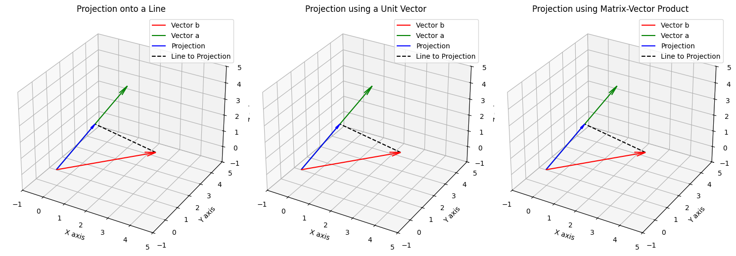
Projection methods in $R^{3}$ (Vector to Vector)#

Projection of Vector $\vec{b} = [4, 1, 2]$ onto $\vec{a} = [1, 4, 3]$ #

Method 1: Projection onto a Line#

The projection of $\vec{b}$ onto $\vec{a}$ is calculated as:

{Proj}_{a} (\vec{b}) = (\frac{\vec{b} \cdot \vec{a}}{\vec{a} \cdot \vec{a}}) \vec{a}

Steps:#

Dot product $\vec{b} \cdot \vec{a}$ :

\vec{b} \cdot \vec{a} = (4) (1) + (1) (4) + (2) (3) = 4 + 4 + 6 = 14

Dot product $ $\vec{a} \cdot \vec{a}$ $:

\vec{a} \cdot \vec{a} = (1) (1) + (4) (4) + (3) (3) = 1 + 16 + 9 = 26

Calculate scalar $β$ :

β = \frac{14}{26} = \frac{7}{13}

Final projection:

{Proj}_{a} (\vec{b}) = \frac{7}{13} \cdot [1, 4, 3] = [\frac{7}{13}, \frac{28}{13}, \frac{21}{13}] \approx [0.54, 2.15, 1.62]

Method 2: Projection Using a Unit Vector#

Normalize $\vec{a}$ :

‖ \vec{a} ‖ = \sqrt{(1)^{2} + (4)^{2} + (3)^{2}} = \sqrt{1 + 16 + 9} = \sqrt{26}

\hat{u} = \frac{1}{\sqrt{26}} [1, 4, 3]

Dot product $\vec{b} \cdot \hat{u}$ :

\vec{b} \cdot \hat{u} = 4 \cdot \frac{1}{\sqrt{26}} + 1 \cdot \frac{4}{\sqrt{26}} + 2 \cdot \frac{3}{\sqrt{26}} = \frac{4 + 4 + 6}{\sqrt{26}} = \frac{14}{\sqrt{26}}

Final projection:

{Proj}_{a} (\vec{b}) = (\frac{14}{\sqrt{26}}) \cdot (\frac{1}{\sqrt{26}}, \frac{4}{\sqrt{26}}, \frac{3}{\sqrt{26}}) = [\frac{14}{26}, \frac{56}{26}, \frac{42}{26}] = [\frac{7}{13}, \frac{28}{13}, \frac{21}{13}] \approx [0.54, 2.15, 1.62]

Method 3: Projection as a Matrix-Vector Product#

Unit vector $\hat{u}$ (as calculated earlier):

\hat{u} = [\frac{1}{\sqrt{26}}, \frac{4}{\sqrt{26}}, \frac{3}{\sqrt{26}}]

Construct the projection matrix ( A ):

\begin{array}{r} A = [\begin{array}{c} u_{1}^{2} & u_{1} u_{2} & u_{1} u_{3} \\ u_{1} u_{2} & u_{2}^{2} & u_{2} u_{3} \\ u_{1} u_{3} & u_{2} u_{3} & u_{3}^{2} \end{array}] = [\begin{array}{c} {(\frac{1}{\sqrt{26}})}^{2} & (\frac{1}{\sqrt{26}}) (\frac{4}{\sqrt{26}}) & (\frac{1}{\sqrt{26}}) (\frac{3}{\sqrt{26}}) \\ (\frac{4}{\sqrt{26}}) (\frac{1}{\sqrt{26}}) & {(\frac{4}{\sqrt{26}})}^{2} & (\frac{4}{\sqrt{26}}) (\frac{3}{\sqrt{26}}) \\ (\frac{3}{\sqrt{26}}) (\frac{1}{\sqrt{26}}) & (\frac{3}{\sqrt{26}}) (\frac{4}{\sqrt{26}}) & {(\frac{3}{\sqrt{26}})}^{2} \end{array}] \end{array}

Matrix multiplication:

\begin{array}{r} A \vec{b} = A [\begin{array}{c} 4 \\ 1 \\ 2 \end{array}] = [\begin{array}{c} \frac{4 + 4 + 6}{26} \\ \frac{16 + 16 + 24}{26} \\ \frac{12 + 12 + 18}{26} \end{array}] = [\begin{array}{c} \frac{14}{26} \\ \frac{56}{26} \\ \frac{42}{26} \end{array}] = [\begin{array}{c} \frac{7}{13} \\ \frac{28}{13} \\ \frac{21}{13} \end{array}] \approx [0.54, 2.15, 1.62] \end{array}

Final Result#

For all three methods, the projection of $\vec{b} = [4, 1, 2]$ onto $\vec{a} = [1, 4, 3]$ is:

{Proj}_{a} (\vec{b}) = [\frac{7}{13}, \frac{28}{13}, \frac{21}{13}] \approx [0.54, 2.15, 1.62]

These methods confirm the correctness of the projection result in $R^{3}$ .

Projection methods in $R^{3}$ implementation in python (Vector to Vector)#

import numpy as np
import matplotlib.pyplot as plt
from mpl_toolkits.mplot3d import Axes3D

# Define the vectors
b = np.array([4, 1, 2])
a = np.array([1, 4, 3])

# Method 1: Projection onto a Line
def projection_line(b, a):
    return (np.dot(b, a) / np.dot(a, a)) * a

proj_line = projection_line(b, a)

# Method 2: Projection Using a Unit Vector
def projection_unit(b, a):
    u = a / np.linalg.norm(a)  # Normalize a
    return np.dot(b, u) * u

proj_unit = projection_unit(b, a)

# Method 3: Projection as a Matrix-Vector Product
def projection_matrix(b, a):
    u = a / np.linalg.norm(a)  # Normalize a
    projection_matrix = np.outer(u, u)  # Outer product to form the matrix
    return projection_matrix @ b  # Matrix-vector multiplication

proj_matrix = projection_matrix(b, a)

# Prepare the figure
fig = plt.figure(figsize=(15, 5))

# Plot Method 1: Direct Projection
ax1 = fig.add_subplot(131, projection='3d')
ax1.quiver(0, 0, 0, b[0], b[1], b[2], color='r', label='Vector b', arrow_length_ratio=0.1)
ax1.quiver(0, 0, 0, a[0], a[1], a[2], color='g', label='Vector a', arrow_length_ratio=0.1)
ax1.quiver(0, 0, 0, proj_line[0], proj_line[1], proj_line[2], color='b', label='Projection', arrow_length_ratio=0.1)

# Dashed line from b to the projection point
ax1.plot([b[0], proj_line[0]], [b[1], proj_line[1]], [b[2], proj_line[2]], 'k--', label='Line to Projection')

ax1.set_xlim([-1, 5])
ax1.set_ylim([-1, 5])
ax1.set_zlim([-1, 5])
ax1.set_title('Projection onto a Line')
ax1.set_xlabel('X axis')
ax1.set_ylabel('Y axis')
ax1.set_zlabel('Z axis')
ax1.legend()

# Plot Method 2: Using a Unit Vector
ax2 = fig.add_subplot(132, projection='3d')
ax2.quiver(0, 0, 0, b[0], b[1], b[2], color='r', label='Vector b', arrow_length_ratio=0.1)
ax2.quiver(0, 0, 0, a[0], a[1], a[2], color='g', label='Vector a', arrow_length_ratio=0.1)
ax2.quiver(0, 0, 0, proj_unit[0], proj_unit[1], proj_unit[2], color='b', label='Projection', arrow_length_ratio=0.1)

# Dashed line from b to the projection point
ax2.plot([b[0], proj_unit[0]], [b[1], proj_unit[1]], [b[2], proj_unit[2]], 'k--', label='Line to Projection')

ax2.set_xlim([-1, 5])
ax2.set_ylim([-1, 5])
ax2.set_zlim([-1, 5])
ax2.set_title('Projection using a Unit Vector')
ax2.set_xlabel('X axis')
ax2.set_ylabel('Y axis')
ax2.set_zlabel('Z axis')
ax2.legend()

# Plot Method 3: Matrix-Vector Product
ax3 = fig.add_subplot(133, projection='3d')
ax3.quiver(0, 0, 0, b[0], b[1], b[2], color='r', label='Vector b', arrow_length_ratio=0.1)
ax3.quiver(0, 0, 0, a[0], a[1], a[2], color='g', label='Vector a', arrow_length_ratio=0.1)
ax3.quiver(0, 0, 0, proj_matrix[0], proj_matrix[1], proj_matrix[2], color='b', label='Projection', arrow_length_ratio=0.1)

# Dashed line from b to the projection point
ax3.plot([b[0], proj_matrix[0]], [b[1], proj_matrix[1]], [b[2], proj_matrix[2]], 'k--', label='Line to Projection')

ax3.set_xlim([-1, 5])
ax3.set_ylim([-1, 5])
ax3.set_zlim([-1, 5])
ax3.set_title('Projection using Matrix-Vector Product')
ax3.set_xlabel('X axis')
ax3.set_ylabel('Y axis')
ax3.set_zlabel('Z axis')
ax3.legend()

# Show the plots
plt.tight_layout()
plt.show()

../_images/fe5618bdd8230d572a3c973122e79a4be9629ceee21a5d9f07cb464ca797a568.png

Definition of Projection in $R^{n}$ #

The projection of a vector $\vec{b} \in R^{n}$ onto the column space of a matrix $A \in R^{n \times m}$ is the vector in the column space of $A$ that is closest to $\vec{b}$ in terms of Euclidean distance. This projection minimizes the difference between $\vec{b}$ and the vector $A \vec{x}$ , where $\vec{x} \in R^{m}$ is the solution to the least squares problem.

Mathematical Expression:#

The projection of $\vec{b}$ onto the column space of $A$ is given by:

{Proj}_{A} (\vec{b}) = A (A^{T} A)^{- 1} A^{T} \vec{b}

where:

$A^{T} A$ is the Gram matrix, representing the inner products of the columns of $A$ ,
$(A^{T} A)^{- 1}$ is the inverse of the Gram matrix (if it exists),
$A^{T} \vec{b}$ is the projection of $\vec{b}$ onto the rows of $A$ .

Geometric Interpretation:#

The resulting vector ${Proj}_{A} (\vec{b})$ lies in the column space of $A$ , meaning it can be expressed as a linear combination of the columns of $A$ . This projection ensures that the residual vector $\vec{b} - {Proj}_{A} (\vec{b})$ is orthogonal to the column space of $A$ .

Key Characteristics:#

The projection minimizes the distance between $\vec{b}$ and the column space of $A$ .
The residual $\vec{b} - A \vec{x}$ is orthogonal to the column space of $A$ .
This method is used in solving least squares problems, where the system $A \vec{x} = \vec{b}$ may have no exact solution due to being overdetermined (more equations than unknowns).

Applications:#

Least squares regression, fitting a model to data points.
Dimensionality reduction, projecting high-dimensional data into a lower-dimensional subspace.

What is Projection?

Contents

What is Projection?#

Definition of Projection in $R^{2}$ #

Projection Derivation#

Projection methods in $R^{2}$ (vector to vector)#

Projection of Vector $\vec{b} = [4, 1]$ onto $\vec{a} = [1, 4]$ #

Method 1: Projection onto a Line#

Method 2: Projection Using a Unit Vector#

Method 3: Projection as a Linear Transformation#

Final Result#

Projection methods in $R^{2}$ implementation in python#

Projection methods in $R^{3}$ (Vector to Vector)#

Projection of Vector $\vec{b} = [4, 1, 2]$ onto $\vec{a} = [1, 4, 3]$ #

Method 1: Projection onto a Line#

Steps:#

Method 2: Projection Using a Unit Vector#

Method 3: Projection as a Matrix-Vector Product#

Final Result#

Projection methods in $R^{3}$ implementation in python (Vector to Vector)#

Definition of Projection in $R^{n}$ #

Mathematical Expression:#

Geometric Interpretation:#

Key Characteristics:#

Applications:#

References#

What is Projection?

Contents

What is Projection?#

Definition of Projection in R2#

Projection Derivation#

Projection methods in R2 (vector to vector)#

Projection of Vector b→=[4,1] onto a→=[1,4]#

Method 1: Projection onto a Line#

Method 2: Projection Using a Unit Vector#

Method 3: Projection as a Linear Transformation#

Final Result#

Projection methods in R2 implementation in python#

Projection methods in R3 (Vector to Vector)#

Projection of Vector b→=[4,1,2] onto a→=[1,4,3]#

Method 1: Projection onto a Line#

Steps:#

Method 2: Projection Using a Unit Vector#

Method 3: Projection as a Matrix-Vector Product#

Final Result#

Projection methods in R3 implementation in python (Vector to Vector)#

Definition of Projection in Rn#

Mathematical Expression:#

Geometric Interpretation:#

Key Characteristics:#

Applications:#

References#

Definition of Projection in $R^{2}$ #

Projection methods in $R^{2}$ (vector to vector)#

Projection of Vector $\vec{b} = [4, 1]$ onto $\vec{a} = [1, 4]$ #

Projection methods in $R^{2}$ implementation in python#

Projection methods in $R^{3}$ (Vector to Vector)#

Projection of Vector $\vec{b} = [4, 1, 2]$ onto $\vec{a} = [1, 4, 3]$ #

Projection methods in $R^{3}$ implementation in python (Vector to Vector)#

Definition of Projection in $R^{n}$ #